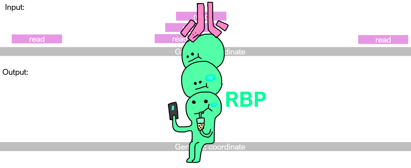
Where does the RNA-binding protein bind!!

December 22, 2020 | 9 Minute Read

What is CLIP-seq?

CLIP-seq is a technology to find where in RNA a certain RNA-binding protein binds. The way we detect this is by crosslinking the protein to the RNA with UV light, then use some antibody to seperate the protein (and the RNA crosslinked to it). By sequencing the RNA fragments purified along with the protein, we can know where that protein binds.

What is Peak Calling?

It is like the reverse problem of the experiment.

Given sequencing reads mapped to the genome, tell me where the protein binds.

What Information do I have?

1. Enriched coverage: The region with more reads are more likely to be bound by protein.

2. Crosslinking events: Also, the crosslinking site on the RNA will intronduce different types of “diagnostic events”, depending on different variants of CLIP-seq. For example, PAR-CLIP crosslink sites is commonly associated with C->T mutation. eCLIP and iCLIP has mostly truncation. HITS-CLIP has deletion at the crosslinking sites. Therefore, by finding those diagnostic events, we can have near-nucleotide resolution to those protein binding sites.

The Naive Peak Calling Tool

Okay. This peak calling problem sounds so easy! Let’s make a sliding 10 nt window, and call a binding site when ever there’s more than 20 reads!

Why It Won’t Work

1. Sequecing data is noisy. Although CLIP-seq protocol has numerous stringent washing steps, in the library there will still be some nonspecific RNAs. Thus, there will be reads that are not from real crosslinking events. That is why we cannot confidently assign every read to a binding event. This problem becomes worse when the RBP binds little target. Compare to the small amount of “real bound RNA”, any abundant transcript like snoRNAs will probably look like peaks.
2. Non-uniform coverage: Unlike ChIP-seq, where each DNA region has equal amount of template, RNA expression is not uniform. The highly expressed can have more reads than the lowly expressed. Therefore, the number of reads at each region is not sufficient to predict protein binding, as it can just reflect high expression. Even within the same RNA, the coverage isn’t uniform either. The GC content of a region can introduce bias in sequencing. Also, spliced intron are degraded (has less template), and therefore has less converage compared to the exons of the same RNA.

Backgrounds are estimated by Size-Matched Input (SMInput) in eCLIP

To tackle the above mentioned problems, eCLIP-seq, the improved version of iCLIP, comes with a “size-matched input”. Size-matched input is generated during the eCLIP experiment, with almost the same steps but without IP-ing the RNA-binding protein of interest. The term “size-matched” come from the gel electrophoresis step, where the RNAs are extracted from the gel with the same size range of the IP. It picks up RNAs rather non-specifically, and thus reflect which RNA is more expressed, thus controls for non-uniform coverage and non-specific background signal. Since it has gone through almost the same steps, it also picks up inherent bias in crosslinking (btw, proteins loves to crosslink to Us due to some mysterious local chemistry), RT-PCR and every step of library prep. By comparing the IP library(RBP) to the input library(background), we now have more information to infer where exactly RBP binds.

The ENCODE eCLIP standard pipeline: CLIPper + Input normalization

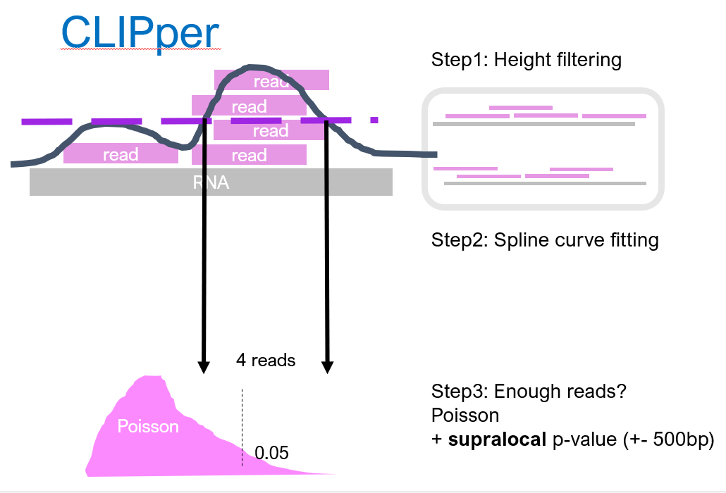
CLIPper[2] is initially designed for iCLIP (where there is no size-matched input). To estimate the background, CLIPper shuffles all reads in a RNA around for 100 times (in reality maybe more). As you can imagine, if there were some regions with peaky coverage, after this shuffling it is gone. The 100 times shuffling generates an empirical probability distribution (the null), describing solely from the background, the probability to observe $n$ reads. Then, we look back at the real data, the unshuffled coverage, and find low probability regions (that is low p-value) where the background distribution cannot explain its coverage. Since the background is estimated seperatly for each RNA, this method controls for uneven gene expression.

Putting it into statistical terms: CLIPper does a permutation testing on coverage.

Then, CLIPper further filters the called regions with the numbers of reads within. It determines the boundary of the peak by spline curve fitting. This time, the number of reads that can appear in background is modelled by Poission distribution. The rate of Poission distribution is estimated from local 500 bp window, so that intronic regions can have its own estimation. Again, regions with sufficient reads (and thus low probability according to the Poisson) will stay and be assigned as a binding site.

CLIPper uses only the IP library, and by multistage filtering, generates a list of peaks. It performs well on a number of RNA-binding proteins. CLIPper tends to call LOTs of peaks.

The statistical testing described above, made an assumption: Only a small portion of reads come from binding, and therefore we can model the background using the rest. If this assumption does not hold true, likely will be falsely estimate the background and failed to capture binding. Examples are ribosomal proteins, where it binds nearly all expressed exons, which is a lot.

With SMInput, the peaks (regions found by CLIPper) is further normalized by SMInput. This uses the data-estimated background to further filter for real peaks. By calculating fold change, peaks that are not enriched can be tossed away. After this filtering, the peaks way more specific.

Other Tools

There are a lot more tools after CLIPper, that look closer to find an appropriate probability distribution to use, and integrate the SMInput as a covariate. For example, the tool Pirahna[5] found that zero-truncated negative binomial(ZTNB) fits better for most RNA-binding proteins at the time. It also allows the SMInput to modify the parameters of ZNTB. For example, in regions that has low SMInput reads (might be due to low expression), the probability of observing 10 reads just from background is lower than a region with lots of SMInput reads, and thus, the shape of ZNTB should be motified. OmniCLIP[6] and PureCLIP[7], other the other hand, uses Hidden Markov Model, allow states (peak or not) to compete, and see which explains the data best. They added even more covariates in the model, including region type(exon, or not), and crosslinking bias (crosslinking motif score). There are even more tools that employs more sophisticated signal processing and new algorithms. For example, WavClusteR originally uses wavelet transformation to call peaks on PAR-CLIP data[8]. But in their later version, the transformation is replaced by a Bayesian Network Approach[9].

So Where Exactly does RNA-binding Proteins Bind?

Okay, enough of math!

The exact position of binding sites, remain a mystery, despite so many efforts. There are many reasons. First, CLIP gives us near-nucleotide resolution, but according to a recent paper[4], it still can be ~20nt off from the real binding site, because crosslinking doesn’t always happen at RNA binding domains. RNA crosslinking requires certain local chemistry (certain amino acid and RNA base) to happen. So for every protein, probably the distance from crosslinking to binding sites differs. Second, the ENCORE projects CLIPped ~150 RNA binding proteins[3], but some of them have very few peaks. There certainly are unsolved issues in the peak calling process. Moreover, even those proteins with good peak calling, the peak is still 50-150 b.p. long, while the canonical RNA-binding site motif usually is 5-20 bp wide. With regards to resolution, improvements are needed.

I think, there are two challenges with regards to the development of a binding site finder. First, RNA-binding proteins is a very heterogenous group. Some bind very few targets (SLBP), some has lot of targets (U2AF1). Some binds widely (Ribosome) while others are narrow. Some has sequence determinants while others don’t. The heterogenity make me wonder if there would ever exist a peak calling tool that works in ALL of them. Second, we lack a goldstandard benchmark to evalute the set of tools. Certainly there are a few well-studied that has high confident binding sites in a few transcripts. But are they comprehensive enough to evaluate tools that aims to draw transcriptomic-wide conclusion? Right now, all we have are indirect evidence (motifs, functional consequences upon knockdown), and none of them are applicable to all RNA binding proteins. To solve this problem, not only computational improvement, but also technology improvements are needed.

A Good Review to Read about CLIP Analysis

Chakrabarti, A. M., Haberman, N., Praznik, A., Luscombe, N. M., & Ule, J. (2018). Data Science Issues in Studying Protein–RNA Interactions with CLIP Technologies. Annual Review of Biomedical Data Science, 1(1), 235–261. https://doi.org/10.1146/annurev-biodatasci-080917-013525

References

1. Van Nostrand, E. L., Pratt, G. A., Shishkin, A. A., Gelboin-Burkhart, C., Fang, M. Y., Sundararaman, B., Blue, S. M., Nguyen, T. B., Surka, C., Elkins, K., Stanton, R., Rigo, F., Guttman, M., & Yeo, G. W. (2016). Robust transcriptome-wide discovery of RNA-binding protein binding sites with enhanced CLIP (eCLIP). Nature Methods, 13(6), 508–514. https://doi.org/10.1038/nmeth.3810
2. Yeo, G. W., Coufal, N. G., Liang, T. Y., Peng, G. E., Fu, X.-D., & Gage, F. H. (2009). An RNA code for the FOX2 splicing regulator revealed by mapping RNA-protein interactions in stem cells. Nature Structural & Molecular Biology, 16(2), 130–137. https://doi.org/10.1038/nsmb.1545
3. Van Nostrand, E. L., Freese, P., Pratt, G. A., Wang, X., Wei, X., Xiao, R., Blue, S. M., Chen, J.-Y., Cody, N. A. L., Dominguez, D., Olson, S., Sundararaman, B., Zhan, L., Bazile, C., Bouvrette, L. P. B., Bergalet, J., Duff, M. O., Garcia, K. E., Gelboin-Burkhart, C., … Yeo, G. W. (2020). A large-scale binding and functional map of human RNA-binding proteins. Nature, 583(7818), 711–719. https://doi.org/10.1038/s41586-020-2077-3
4. Corley, M., Flynn, R. A., Lee, B., Blue, S. M., Chang, H. Y., & Yeo, G. W. (2020). Footprinting SHAPE-eCLIP Reveals Transcriptome-wide Hydrogen Bonds at RNA-Protein Interfaces. Molecular Cell, 80(5), 903-914.e8. https://doi.org/10.1016/j.molcel.2020.11.014
5. Uren, P. J., Bahrami-Samani, E., Burns, S. C., Qiao, M., Karginov, F. V., Hodges, E., Hannon, G. J., Sanford, J. R., Penalva, L. O. F., & Smith, A. D. (2012). Site identification in high-throughput RNA–protein interaction data. Bioinformatics, 28(23), 3013–3020. https://doi.org/10.1093/bioinformatics/bts569
6. Drewe-Boss, P., Wessels, H.-H., & Ohler, U. (2018). omniCLIP: Probabilistic identification of protein-RNA interactions from CLIP-seq data. Genome Biology, 19(1), 183. https://doi.org/10.1186/s13059-018-1521-2
7. Krakau, S., Richard, H., & Marsico, A. (n.d.). PureCLIP: capturing target-specific protein-RNA interaction footprints from single-nucleotide CLIP-seq data. 27.
8. Sievers, C., Schlumpf, T., Sawarkar, R., Comoglio, F., & Paro, R. (2012). Mixture models and wavelet transforms reveal high confidence RNA-protein interaction sites in MOV10 PAR-CLIP data. Nucleic Acids Research, 40(20), e160. https://doi.org/10.1093/nar/gks697
9. Comoglio, F., Sievers, C., & Paro, R. (2015). Sensitive and highly resolved identification of RNA-protein interaction sites in PAR-CLIP data. BMC Bioinformatics, 16(1), 32. https://doi.org/10.1186/s12859-015-0470-y